Welcome to Bank Marketing Example

An Adoption of AI in banking has become more of a necessity rather than a choice. One of the most common use cases is predictive analytics. AI-driven predictive marketing methods are deployed by many financial institutions to detect specific patterns and correlations of the data. These patterns in turn provide meaningful insights indicating the target groups, the untapped sales opportunities, etc.

This example will investigate the bank marketing dataset shared here which is related to direct marketing campaigns (telemarketing) of a Portuguese banking institution. The objective of this example is to predict whether the client will subscribe to a term deposit. This dataset contains 16 variables and is ordered by date from May 2008 to November 2010. The dataset contains 45,211 elements, which I split into 90:10 for training and unseen data.

Data exploration

To understand the problem, I first carefully check the dataset information. The dataset contains 16 variables as listed below:

Input variables	bank client data
age	age of the client
job	type of job
marital	marital status
education	educational level
default	whether the customer has credit in default.
balance	balance of the client
housing	whether the customer has a housing loan
loan	whether the client has a personal loan

| contact | contact communication type (cellular, telephone) | | month | last contact month of years ( January - December) | | day of weeks | last contact day of the week | | ~~duration~~ | ~~last contact duration in seconds~~ | | campaign | numbers of contacts performed during this campaign and for this client | | pdays | numbers of days that passed by after the client was last contacted from a previous campaign | | previous | numbers of contacts performed before this campaign and for this client | | poutcome | outcome of the previous marketing campaign | | y | whether the client has subscribed term deposit. |

As stated in the dataset document, one attribute ('duration') should be excluded. This attribute highly affects the output target meaning that if the duration is "0", then the value y is "no". The duration value is not known until the call is performed. However, once the call is made, the value of y will be known. Therefore, it is recommended to eliminate this attribute before building a model.

Moreover, I split 10% of the dataset into unseen data for the models' performance evaluation at a later stage.

Handling an Unknown Value

Although the dataset has no Nan or null value, the categorical data contain unknown values including job, education, and contact. The unknown values can also be treated as another class label to provide the model with more information on the data. Here, I replace the unknown value with a mode for job and education. I keep the unknown value for the contact attribute since it has a higher proportion and it can be biased to just fill the value with mode.

---

Before	After
---

Handling Categorical and Ordinal Variables

Let's explore the training set further. This dataset contains both numerical and categorical variables. To build an ML model, it is compulsory to transform categorical into numeric features. I perform one-hot-encoding on categorical variables. The ordinal features (day and month) are encoded with cyclical encoding to preserve the cyclical structure by applying sin and cos functions. The below figure demonstrates an example of cyclical encoding on the day and month features.

Month	Day

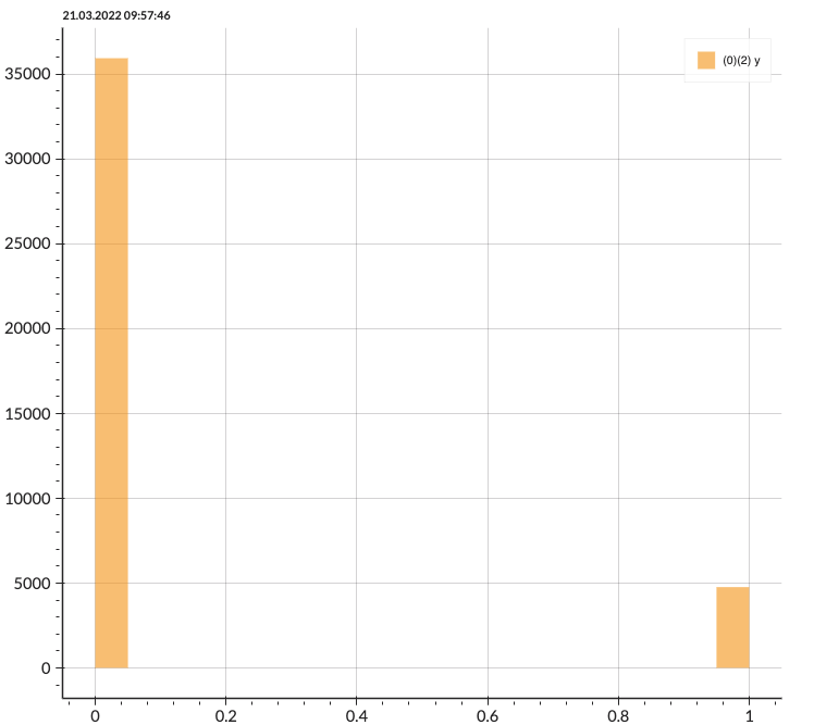
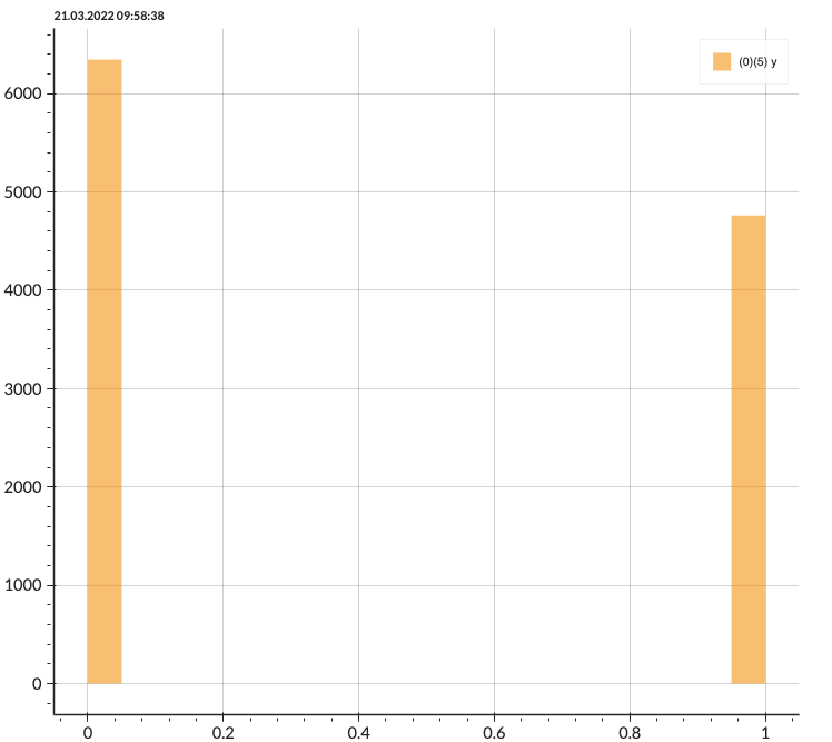
Handling an Imbalanced Data

Before training the model, I resample the training set due to the imbalance of the data. Here, I perform 75% of the Near Miss under-sampling technique to introduce more balance into the dataset. (Note: 100% Under-sampling can distort the information of the data, therefore I chose to decrease the data by only 75%.)

Before	After

Correlation

Let's now take a look at the relationship between attributes! The correlation, unfortunately, does not have a strong or weak correlation in which we can drop some features, ideally, when the correlation score is less than -0.8. As a result, we will train with all attributes presented.

Attribute	Value	Attribute	Value	Attribute	Value	Attribute	Value
age	-0.02	job	0.04	contact	-0.15	month	0.02
marital	0.05	education	0.07	pdays	0.11	campaign	-0.07
default	-0.02	housing	-0.14	previous	0.09	poutcome	-0.08
loan	-0.07	balance	0.05	day	-0.03

Data Modeling and Test Results

Metrics

For an imbalanced dataset, we need to consider balanced accuracy rather than classification. A model can have high accuracy with bad performance, or low accuracy with better performance, in which we need to consider different criteria of metrics.

Here we introduce different types of metrics used in classification as follows;

Precision: The number of true positives divided by all positive predictions.

Recall: The number of true positives divided by the number of positive values in test data.

F1: The weighted average of precision and recall.

ROC-AUC: The curve created by plotting true positive rate against false positive rate, in which the area under the curves can tell how good the model is.

Balanced Accuracy: A metric that one can use when evaluating how good a binary classifier is.

(NOTE: In our example, where the majority is negative, balanced accuracy is the metric we should base on.)

Training Model \& Results

Choosing models for imbalanced data can help with the model performance. For example, boosting models can give more weight to the cases that get misclassified, which are more suitable for an imbalanced dataset than the simple models such as logistic regression. The training data is separated again into 70:15:15 for train, validation, and test sets. The results demonstrated in the following tables are evaluated on unseen data (separated at the beginning). I train the models with two options including

1. Without under-sampling technique.
2. With Near Miss undersampling of 75%.

For both cases, three models are trained including GradientBoosting (GB), Bagging, AdaBoosting (Ada), XGBoost (XGB).

Below the figure is the results from model 1 where I train without under-sampling. The results show a good score on the classification accuracy, but not the rest. The reasons behind are mentioned earlier that classification accuracy might not be able to describe how good the model is for an imbalanced dataset.

	Model	Accuracy	Precision	Recall	F1	ROC	Balanced Accuracy
	GB	0.893	0.699	0.149	0.246	0.57	0.57
1	Bagging	0.891	0.569	0.267	0.363	0.62	0.619
	Ada	0.891	0.622	0.183	0.283	0.584	0.584
	XGB	0.889	0.561	0.217	0.313	0.597	0.597

Now, let's take a look at another result. Below is the result of the model trained with the under-sampling technique. Accuracy is lower than in the aforementioned case, but the balanced accuracy is better for these models. Additionally, this dataset demands attention on the negatives meaning that F1 scores should not be based because F1 is a suitable scoring metric for an imbalanced dataset, in which more attention is needed on the positives.

	Model	Accuracy	Precision	Recall	F1	ROC	Balanced Accuracy
	GB	0.838	0.369	0.537	0.437	0.708	0.708
2	Bagging	0.823	0.343	0.561	0.426	0.71	0.709
	Ada	0.83	0.35	0.526	0.42	0.7	0.7
	XGB	0.841	0.375	0.546	0.445	0.713	0.713

Takeaway Messages & Further Improvement

1. An imbalanced data requires specific techniques for balancing the data before the model implementation such as under-sampling and over-sampling.
2. Metrics need to be selected carefully to evaluate the model correctly. Sometimes, people get trapped with the standard accuracy measurement which cannot best describe the model.
3. Model selection is important because not all models are designed for imbalanced data.
4. Improvement can be done by handling outliers or combining under-sampling and over-sampling techniques.
5. Hyper-parameters tuning can enhance the model's performance.