Welcome to the Mall Customer Segmentation Example
Successful business strategy is built upon an understanding of business target customers. Clustering is one of the powerful methods allowing marketers to visualize and analyze their customers for their further strategy implementation. The mall customer segmentation dataset shared here on Kaggle is created for the learning purpose of customer segmentation to analyze customers to foresee the potential customers who can easily converge. The information is useful for the marketing team and their strategic plan.
Data Exploration
As usual, our first step is to understand the problem by exploring the dataset. This dataset contains information collected from 200 customers and 5 attributes as follows;
| Input Variable | Attributes |
|---|---|
| Customer ID | ID of an individual customer |
| Age | Age of customer |
| Annual Income | Customer's yearly income |
| Spending Score | Score assigned to the customer based on defined parameters. |
| (i.e. customer behavior and purchasing data.) |
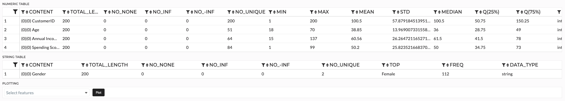
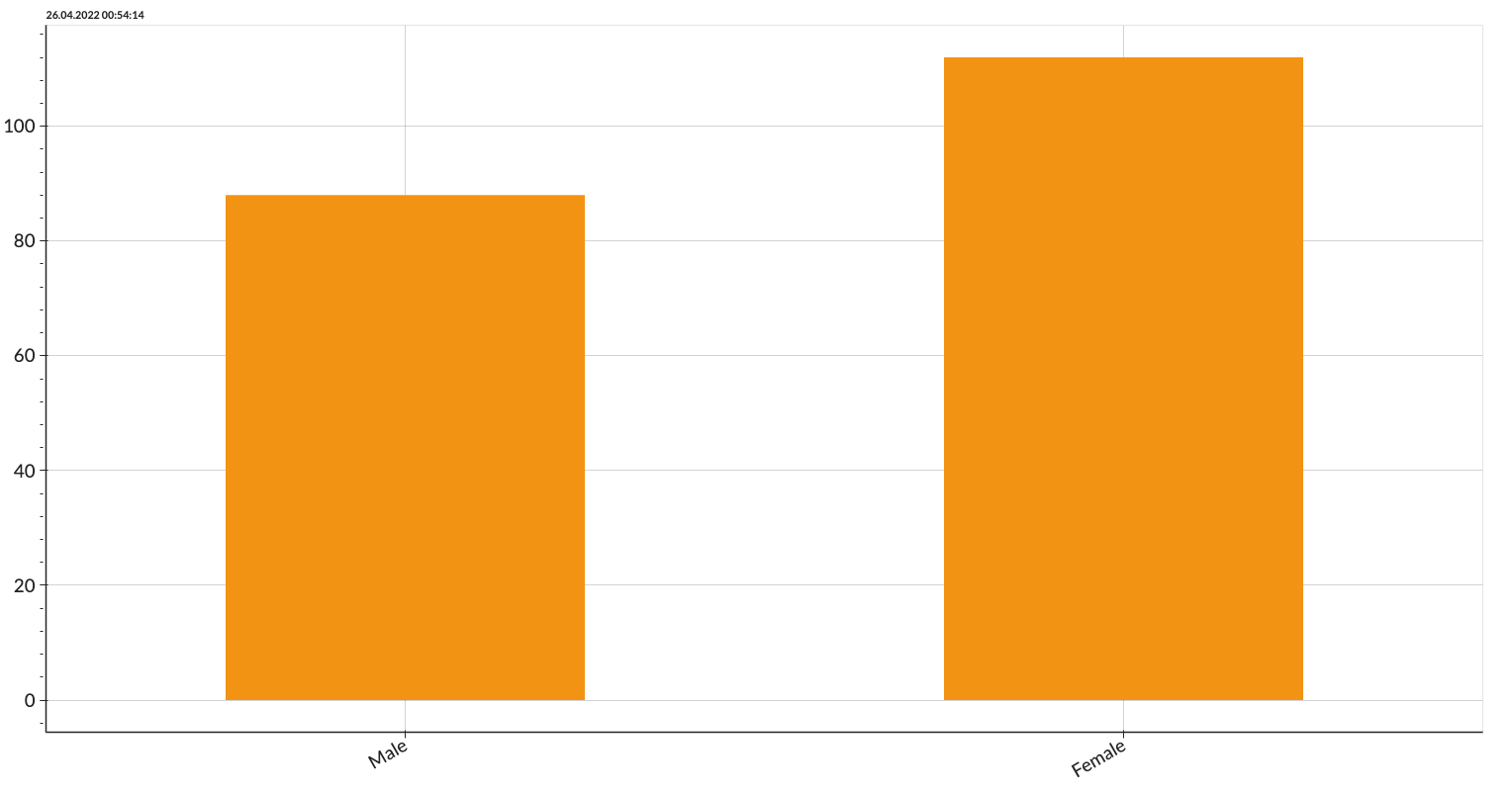
Figure 1 shows a brief overview of the dataset. It can be interpreted that the majority of the mall visitors are female. The minimum and maximum ages of the mall visitors are 18 and 70 respectively. Spending score ranges from 1 to 99 showing a wide range of customers' spending.
This dataset does not contain any missing values. Since the Customer ID is a unique identifier we do not want to include it in clustering. We will drop the Customer ID feature. Now, we will take some time to understand each feature.
| Gender | Age |
|---|---|
 |
 |
| Income | Spending Score |
|---|---|
 |
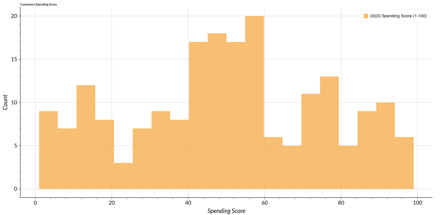 |
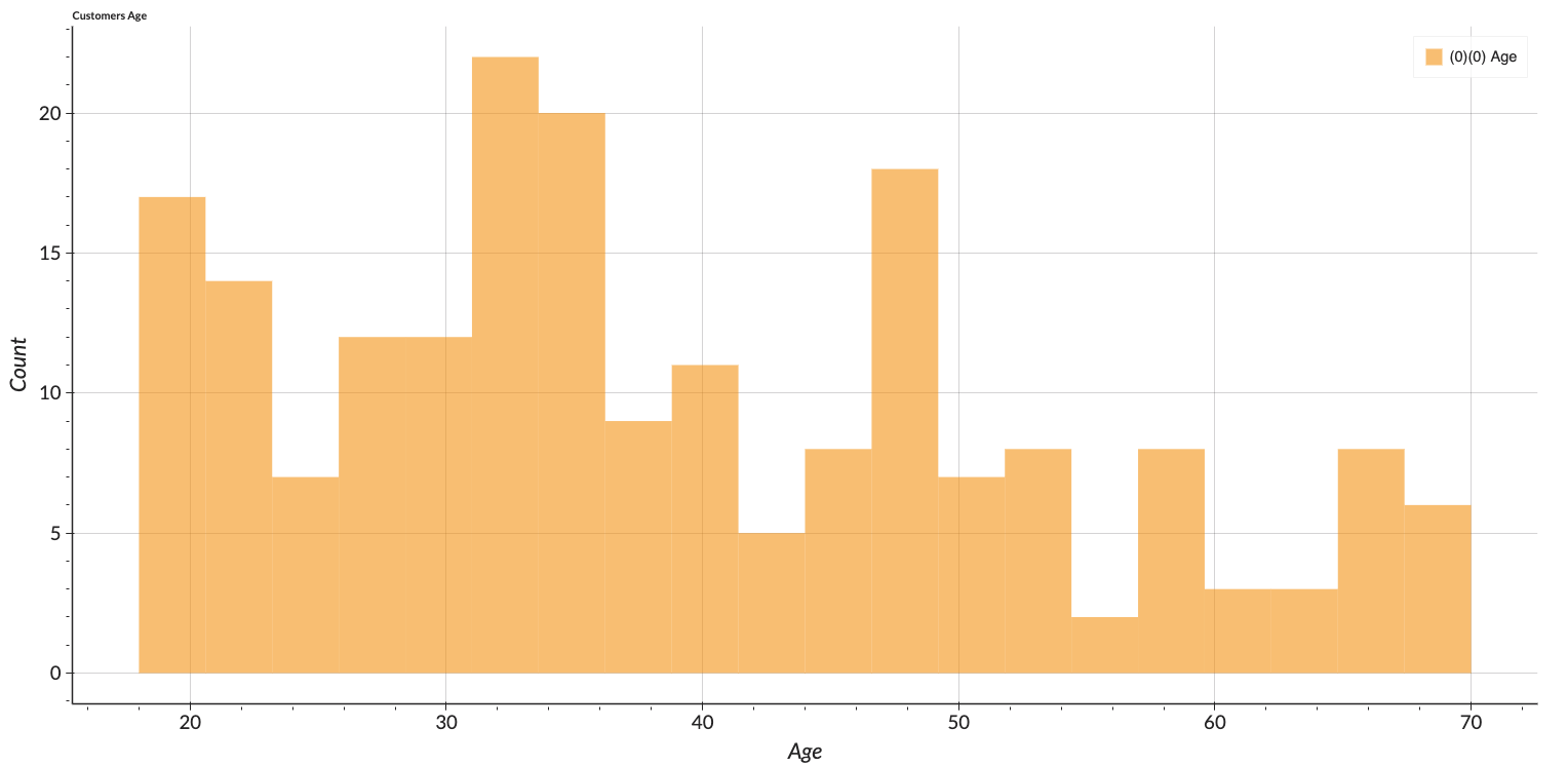
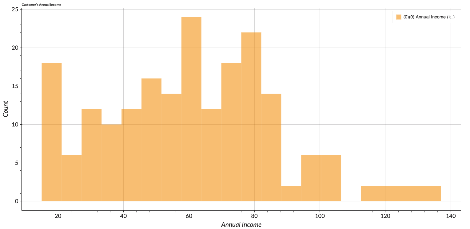
The figures show the distribution of each attribute. Only the income feature is slightly right-skewed. The spending score represents the variety of customers and can be perceived that the malls can meet the various needs of the customers. The customers vary in terms of their annual income and ages. However, we can see that mostly the customers in the age range of 30 to 40 have more engagement than others.
Correlation Score
| Signal | Correlation Score |
|---|---|
| Gender | -0.0581 |
| Age | -0.3272 |
| Annual Income | 0.0099 |
We perform Pearson correlation analysis and report only the score that is correlated to the spending score feature. The age variable is a significant feature with a negative value. In other words, at a higher age, a customer's spending score decreases. Let's see with the correlation viewer for a clearer picture.
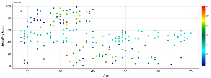
The relationship between the age and the spending score demonstrates the trend in accordant with the correlation score (inversely proportional). The scatter plots are colored regarding the annual income feature. We can notice also that young customers with lower income are likely to spend more.
K-Means Clustering
K-Means is one of the popular unsupervised machine learning algorithms which does not need to refer to any known, labeled outcome. In this example, we will use this method to group similar data points with similar patterns.
The letter K refers to the fixed number of clusters. To perform K-means clustering, K needs to be defined. Luckily, our platform already has this option ready. The number of clusters can either be defined automatically or custom if we would have already fixed the desired K.
In this example, K is defined automatically with four input features fed into the algorithm including age, gender, spending score, and annual income. Let's explore our results!
Data Cluster Analysis
After applying the model, the data points are clustered into four groups being labeled as 0 - 3. The interpretation of the results depends on which features we are looking at.
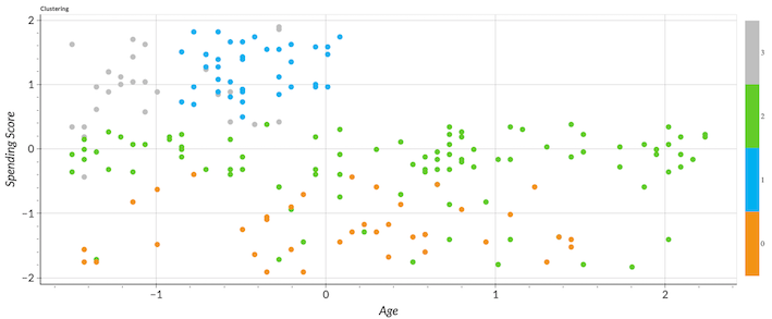
First, we analyze the clusters based on spending score and age.
- Cluster 0 is a group with low to medium age and low spending scores.
- Cluster 1 is a group with low to medium age and high spending scores.
- Cluster 2 is a group with a wider range of age and medium spending scores.
- Cluster 3 is a group with low age and high spending scores.
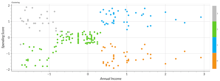
Now, we analyze spending scores against annual income features.
- Cluster 0 is a group with medium to high annual income and low spending scores.
- Cluster 1 is a group with medium to high annual income and high spending scores.
- Cluster 2 is a group with low to medium annual income and low to medium spending scores.
- Cluster 3 is a group with low annual income and high spending scores.
We can interpret the overall result as follows;
- Cluster 0 is a group with low to medium age, medium to high income, and low spending scores.
- Cluster 1 is a group with low to medium age, medium to high income, and high spending scores.
- Cluster 2 is a group with a wider range of age, low to medium income, and low to medium spending scores.
- Cluster 3 is a group with low age, low annual income, and high spending scores.
What kind of insight can be extracted from these clusters?
Well, the goal of this problem is to find the target customers who have a high tendency to converge easily. In this case, cluster 1 is the ideal group that has high spending score and also high income. Cluster 3 are customers with low age who enjoy lives which can be the second most important group of customers.
Moreover, cluster 0 can be seen as potential customers who have high income but the products available at the malls might not be able to answer their needs. From that being said, it is worthwhile to explore a new strategy to tackle this potential group of customers.
However, cluster 2 seems not so clear if they can be left out. They are somehow a mix between low to medium spending scores. Our suggestion is to try a different strategy to define the optimal K value such as the Elbow and Silhouette method. Increasing K value would be beneficial if we want to narrow down the specific target customers.
Summary
Clustering is an unsupervised ML algorithm that can help us to understand the underlying pattern of data points. K-Means is one of the simplest and. The well-known method in clustering data is to deepen the insights. The optimal value of K is crucial for the implementation of the algorithm to tackle the business problem. Most importantly, interpretation of the results needs to be done carefully to extract useful insights from this clustering problem.