Smooth
Smooth TAB enables you to smooth your dataset using different filtering methods. In digital signal processing, smoothing is a function that attempts to capture important patterns in the Signal while simultaneously attenuating the noise or other rapid changes in that Signal. Smoothing aims to produce slow changes in value so that it is easier to see trends in our data. The list of filtering methods is available in the Reference section.
This tutorial assumes that you already selected a project and imported data. For more information please visit on Project and Import Data section.
User Interface Structure
This section helps to familiar with the Smooth TAB interface elements.
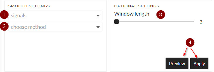
1. Signals
Choose input dataset in the signals (multi-select possible). It can only values type signal or value-vector pairs type signal where value-vector pair means Time-series signal. The vector represents the time axis in Time-series data. If the value-vector pair type signal is selected, the system collects sampling frequency (fs) information from the vector information; otherwise, the system will automatically consider the sampling frequency (fs) as 1.
2. Choose method
Select the desired smooth method that you want to use. There are 16 different options available in the Reference section.
3. Window length
Select the length of Window in the slider. The window size can not be larger than signal length.
4. Preview/Apply
Preview button will do the operation but will not save the data, while Apply will give you the option to save the data in a folder in content. More information is available in here
Basic Usage
Using different Smooth operation is simple, and you need to follow the following steps:
- Choose input datasets in the signals
- Choose a method of smoothing.
- Select the length of Window in the slider.
- Preview/ Apply operation
The following animation shows an example of Moving Mean smoothing using window size as 10:
Filter
In all Data Enrichment Tabs, you can select only a part of the data using a Filter. A more detailed description of Filters can is available here
References
Below is the complete list of available methods:
- Moving Mean: This is a non-weighted moving average of the data. The window size always should be an Odd number.
- Moving Median: A median filter is a nonlinear filter in which each output sample computes as the median value of the input samples under the Window – that is, the result is the middle value after the input values have been sorted. More details is available here.
- Exponential Moving Average: An exponential moving average (EMA) is a type of moving average (MA) that places a greater weight and significance on the most recent data points. The exponential moving average is also referred to as the exponentially weighted moving average. An exponentially weighted moving average reacts more significantly to recent price changes than a simple moving average(SMA), which applies an equal weight to all observations in the period.
- Gaussian: The Gaussian Filter smooths data by acting as a low pass filter to reduce noise (high-frequency components). More details is available here.
- Savitzky-Golay Filtering P2: This method smooths a signal by applying Savitzky-Golay Filtering of polynomial order of 2. More details is available here.
- Savitzky-Golay Filtering P2: This method smooths a signal by applying Savitzky-Golay Filtering of polynomial order of 3. More details is available here.
- Savitzky-Golay Filtering P2: This method smooths a signal by applying Savitzky-Golay Filtering of polynomial order of 4. More details is available here.
-
Savitzky-Golay Filtering P2: This method smooths a signal by applying Savitzky-Golay Filtering of polynomial order of 5. More details is available here.
-
Detrend Signal: This method smoothes the data by removing linear trends. More details is available here.
-
Lowess: Locally Weighted Scatterplot Smoothing (Lowess) is a function that outs smoothed estimates of endog at the given exog values from points (exog, endog). More details is available here.
- Smooth Hanning: This method is based on the convolution of a scaled Hanning window with the Signal. The Signal is prepared by introducing reflected copies of the Signal (with the window size) both ends so that transient parts are minimized in the beginning and end of the output signal.
- Smooth Hamming: This method is based on the convolution of a scaled Hamming window with the Signal. The Signal is prepared by introducing reflected copies of the Signal (with the window size) both ends so that transient parts are minimized in the beginning and end of the output signal.
- Smooth Bartlett: This method is based on a scaled Bartlett window convolution with the Signal. The Signal is prepared by introducing reflected copies of the Signal (with the window size) both ends so that transient parts are minimized in the beginning and end of the output signal.
- Smooth Blackman: This method is based on the convolution of a scaled Blackman window with the Signal. The Signal is prepared by introducing reflected copies of the Signal (with the window size) both ends so that transient parts are minimized in the beginning and end of the output signal.
- ** Exponential Moving Average (EMA):** Provide exponentially weighted (EW) calculations. More details is available here.
- ** Wavelet Smoothing: ** You can do discrete wavelet(DWT) smoothing here. In this method the signal is reconstructred used thresholded DWT components. You can read more about DWT here