Train Model

Train model tab is for training your model with your data. You have several options here to select the model. You can also choose multiple models to train with your data and select the best model from the results.

Image_Caption

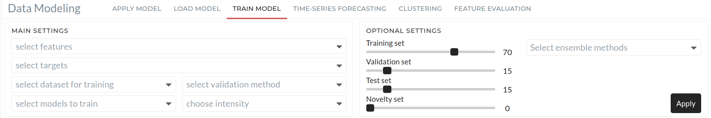
Figure: Train model user interface

Objectives

By the end of this lesson, you will be - familiar with the train model tab and - learn how to use this tab for creating your model.

Note

This tutorial assumes that you have already selected a project and imported data. For more information, please see Import Data section in Getting Started.

Familiarity with the user interface

Train model operation configuration is divided into two main settings. 1. Main settings 2. Optional settings

Main Settings

You must have to select all the options here.

Image_Caption

Figure: Main settings

Select features

All feature data for training the model have to select here.

Select targets

The target for the model has to select here. Target can be more than one. If you choose multiple targets, multiple models will generate for these targets.

Select dataset for training

You can define the percentage of the data you want to select. For example, you may want only 20% of the data during various trials, and in the final run, you want all of the data. This Drop-Down is the place where you can define that.

Select models to train

The target model has to select here. There are lots of model selection options. Here also you can select multiple models. For example, you can select AdaBoost and DecisionTree at the same time. Based on selected models and targets, you will get the results. For example, if you select 2 targets and 2 models, you will get 2x2=4 total models.

Select validation method

You can select the validation method here. Basic split means the normal splits without any folding. No split means all the data will be used for training. You can also use Cross-validation with 3/5/8/10 folds.

Choose intensity

Intensity depends on the validation method. If you choose Basic, you have only one intensity option, Default. - Default - All the algorithms will use their default parameters.

if you choose No Split then you can not choose intensity.

if you choose Cross-Validation, then you have 5 options: - Default - All the algorithms will use their default parameters. - Medium - BayesSearch with selected parameters and number of iteration is 10% of parameter combinations - High Intensity - BayesSearch with all the parameters and number of iteration is 10% of parameter combinations - Higher Intensity - BayesSearch with all the parameters and number of iteration is 25% of parameter combinations - Highest Intensity - GridSearch with all the parameters

Optional settings

Selections are optional here. If not chosen, then default values will use in the configuration.

Image_Caption

Figure: Optional settings

Training set

Default training set is 70% of the data. You can change it according to your required ratio. The slider can be adjusted using a mouse or keyboard. For adjusting small changes, the keyboard is a good choice.

Validation set

Default validation set is 15% of the data. You can change it according to your required ratio.

Test set

Default test set is 15% of the data. You can change it according to your required ratio.

Novelty set

Default Novelty set is 0% of the data. You can change it according to your required ratio.

Select Ensemble Methods

You can select one or more ensemble methods here. Available options are - Stacking - Blending - Voting

If you select any ensemble method, then all the models chosen in the train model Drop-Down will be treated as weak learners models for the selected ensemble method. By default, Logistic Regression uses as the final estimator for classification, and Linear Regression uses as the final estimator for regression.

Note

Must Be: Training set + Validation set + Test set + Novelty set = 100

Apply Configuration

After main settings and optional settings configurations, you must press the Next button. Then apply configuration pop up will appear. You can see the target signal in the regression or classification section. You can also select the error metric here. Default options for regression and classification are r2 score and accuracy. Additionally, if you want to tune the hyperparameters of the selected models, you can select the hyperparameter tuning option.

Image_Caption

Figure: Confirmation of classification or Regression Targets

Start Job

Image_Caption

Figure: Starting Job

By pressing, you can start the job. There are optional configurations here. We have a separate detailed tutorial to learn more about starting a job. You can see the running model status in the window.

Note: Some models take more cores and memory to run. So, it is recommended to run the model jobs with more cores and memory.

Note

The following sections assume that you already know how to use the train model tab. If not, then please learn how to use the train model tab from [above](#train-model)

Classification Example - Iris Species Prediction

Here we will do all the steps .to train a model for predicting iris species. Here we assume that you already have imported the iris data.

Objectives

By the end of this section, you will be - able to create a classification model - able to see the trained model results

Configurations

Main settings configurations.

Main Settings

Image_Caption

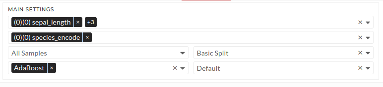
Figure: Train model main settings

Follow these steps: - select feature sepal_length, sepal_width, petal_length and petal_width - select target species_encode - select All Samples in the dataset Drop-Down - select AdaBoost (AdaBoost will be AdaBoost classifier automatically as it is a classification problem) - select Basic Split validation - select Default intensity

Optional Settings

Image_Caption

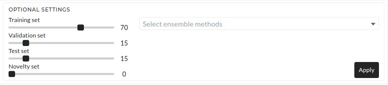
Figure: Train model optional settings

Keep all the default settings as it is in optional settings. All the default values will be used.

Apply Settings

Image_Caption

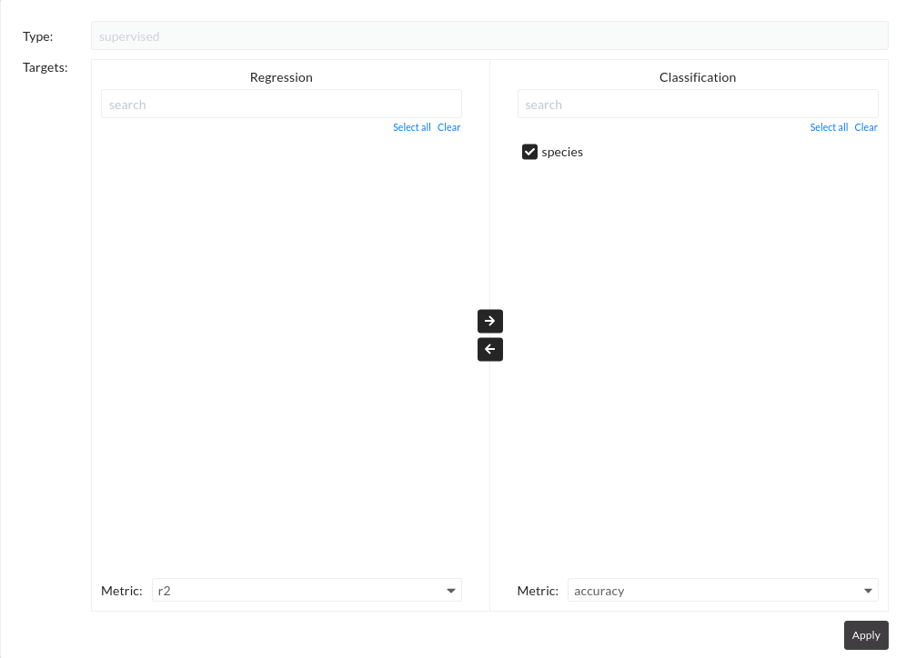
Figure: Train model apply settings

Press Apply. A pop-up window will come, and here, confirm the default settings. Target species will show in the Classification section, and the default error metric will be accuracy. Again press Apply

Start Job Settings

Image_Caption

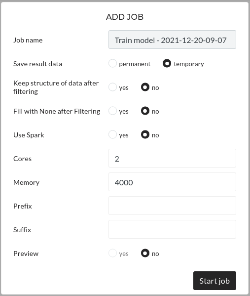
Figure: Train model start job settings

Keep all the default settings and press Start Job.

Results

You will see now in the table that the model is running.

Image_Caption

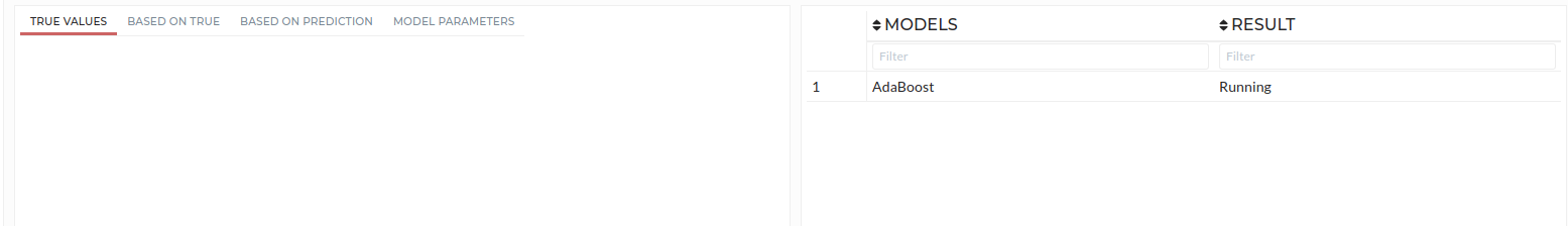
Figure: Train model status

After a few times, the model result will come automatically, and you will see the result like the below image. In your case, the results will be different.

Image_Caption

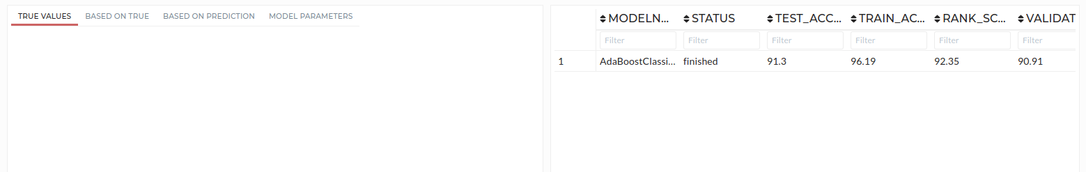
Figure: Train model result

Result Discussions

Image_Caption In the above image, this is an example of the classification result. Here in the table, you can see the model name, train, test and validation, novelty accuracies. Also, based on accuracies, an overall ranking is assigned. The ranking is useful when training of multiple models occurs at the same time.

Click on the model name. You will see a plot on the left side. There are four tabs, and one of these is for the parameter table that displays the trained model’s parameters. True Values’s first plots show the confusion matrix based on True values and Predicted values. The second plot shows the same confusion matrix based on True value percentage. The third plot shows the same confusion matrix based on predicted value percentage.

Understanding Model Training Concepts

Classification

Classification predictive modeling is the task of approximating a mapping function (f) from input variables (X) to discrete output variables (y).

The output variables are often called labels or categories. The mapping function predicts the class or category for a given observation.

For example, an email can be either spam or not spam.

Regression

Regression predictive modeling is the task of approximating a mapping function (f) from input variables (X) to a continuous output variable (y).

A continuous output variable is a real value, such as an integer or floating-point value. These are often quantities, such as amounts and sizes.

For example, a house may be predicted to sell for a specific dollar value, perhaps 200,000.

Confusion Matrix

A confusion matrix is a summary of prediction results on a classification problem. The number of correct and incorrect predictions are summarized with count values and broken down by each class. This is the key to the confusion matrix. The confusion matrix shows how your classification model is confused when it makes predictions.

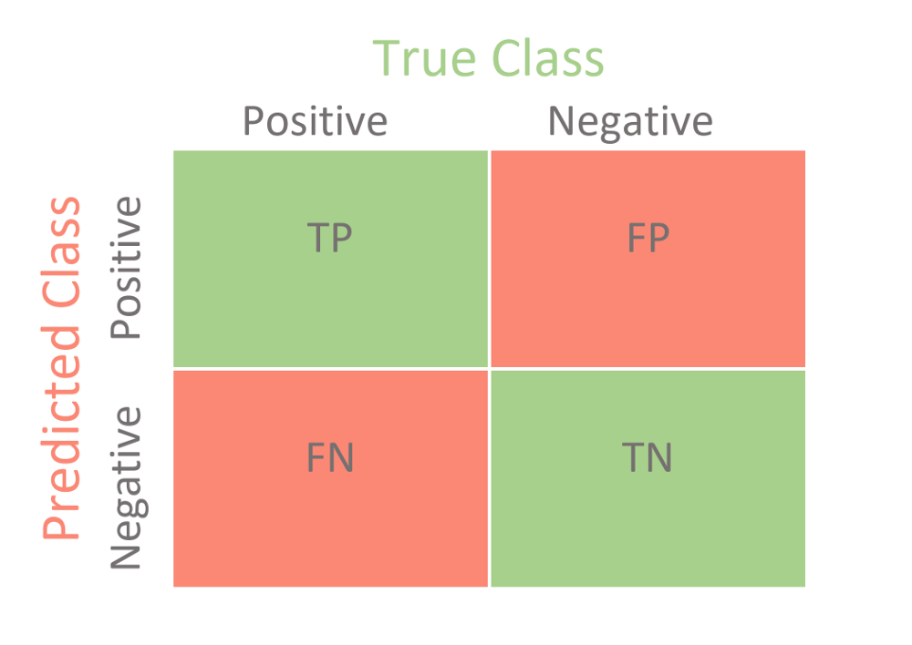
Figure: Confusion Matrix

Scatter Plot

A scatter plot (aka scatter chart, scatter graph) uses dots to represent values for two different numeric variables. The position of each dot on the horizontal and vertical axis indicates values for an individual data point. Scatter plots use to observe relationships between variables.

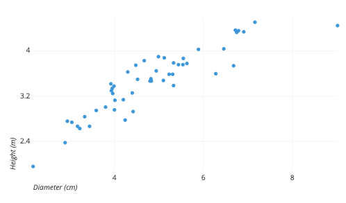
Figure: Scatter Plot

References

XGBRegressor

XGB does not work if your target contains negative values when the hyper-parameter objective is set to 'reg:tweedie'. So if your data contain negative values, please use another model. Or you can use the Default XGB option. That is, you have to select Default in the intensity drop down. Other available options like medium, high, higher, or highest use optimization technique to find the best hyper-parameter combination and tweedie will be one of the options and eventually it will not work because of negative values.

XGBRegressor : read detail from here.

CatBoostRegressor

BernoulliNB : read detail from here.

Q & A

Q. I wanted to use Adaboost classifier, but I found only Adaboost. Is it the same thing?

A. Yes, you can use Adaboost. Internally based on target types Adaboost will be automatically Adaboost classifier if it is a classification problem or it will be Adaboost regressor if it is a regression problem.

Q. What is the difference between classification and regression in Machine Learning?

A. Classification is about predicting a label, and regression is about predicting a quantity.

Q. When will we use novelty?

A. If you think your data contains some irrelevant values, then you can use novelty set.

Q. How should data be divided into train, validation, and test sets?

A. Normally, 70% of the dataset is used for training, 15% for validation, and 15% for testing.

Q. What are the available classification algorithms?

A. Available algorithms are:

AdaBoostClassifier

BaggingClassifier

BernoulliNB

DecisionTreeClassifier

ExtraTreeClassifier

ExtraTreesClassifier

GaussianProcessClassifier

GradientBoostingClassifier

KNeighborsClassifier

LogisticRegression

MLPClassifier

NearestCentroid

PassiveAggressiveClassifier

Perceptron

RandomForestClassifier

RidgeClassifier

SGDClassifier

SVC

LinearDiscriminantAnalysis

GaussianNB

QuadraticDiscriminantAnalysis

XGBClassifier

Q. What are the available regression algorithms?

A. Available algorithms are:

AdaBoostRegressor

BayesianRidge

DecisionTreeRegressor

ElasticNet

ExtraTreesRegressor

ExtraTreeRegressor

GradientBoostingRegressor

HuberRegressor

KNeighborsRegressor

Lars

Lasso

LassoLars

LassoLarsIC

LinearRegression

LinearSVR

MLPRegressor

PLSCanonical

PLSRegression

PassiveAggressiveRegressor

RandomForestRegressor

Ridge

SGDRegressor

SVR

TheilSenRegressor

ARDRegression

CCA

OrthogonalMatchingPursuit

RANSACRegressor

BaggingRegressor

XGBRegressor

CatBoostRegressor

Train Model

Objectives

Familiarity with the user interface

Main Settings

Select features

Select targets

Select dataset for training

Select models to train

Select validation method

Choose intensity

Optional settings

Training set

Validation set

Test set

Novelty set

Select Ensemble Methods

Apply Configuration

Start Job

Classification Example - Iris Species Prediction

Objectives

Configurations

Main Settings

Optional Settings

Apply Settings

Start Job Settings

Results

Result Discussions

Understanding Model Training Concepts

Classification

Regression

Confusion Matrix

Scatter Plot

References

Classification and Regression

AdaBoostClassifier

BaggingClassifier

BernoulliNB

DecisionTreeClassifier

ExtraTreeClassifier

ExtraTreesClassifier

GaussianProcessClassifier

GradientBoostingClassifier

KNeighborsClassifier

LogisticRegression

MLPClassifier

NearestCentroid

PassiveAggressiveClassifier

Perceptron

RandomForestClassifier

RidgeClassifier

SGDClassifier

SVC

LinearDiscriminantAnalysis

GaussianNB

QuadraticDiscriminantAnalysis

XGBClassifier

AdaBoostRegressor

BayesianRidge

DecisionTreeRegressor

ElasticNet

ExtraTreesRegressor

ExtraTreeRegressor

GradientBoostingRegressor

HuberRegressor

KNeighborsRegressor

Lars

Lasso

LassoLars

LassoLarsIC

LinearRegression

LinearSVR

MLPRegressor

PLSCanonical

PLSRegression

PassiveAggressiveRegressor

RandomForestRegressor

Ridge

SGDRegressor

SVR

TheilSenRegressor