Welcome to the Human Activity Recognition Tutorial
One of the most interesting public data science projects is human activity recognition. It is about recognizing various human activities like lying, walking, and sitting with the help of your smartphone device. It even considers differentiating between walking straight, upstairs, and -downstairs. This use case got so famous that it already gained some extensions, like recognizing more activities and with more devices such as smartwatches or tablets. Plus, a good experience with this use-case is that you attend with your smartphone which you will be able to approach the other use-cases yourself.
This demonstration aims to train several Machine Learning (ML) models to classify human activity depending on the given signals correctly. We will derive meaningful features from the raw signals with the Feature Extraction Tab. After establishing a good-performing ML model, we will build a go-live Story and App. Finally, we will collect our measurements and conduct a test with our Model.
Note
We start the use-case from scratch and use the raw signals. However, if you google for the dataset you find often datasets with derived features already and not the original dataset.
For simplicity, let's separate the tutorial into two sections.
-
- Data Acquisition
- Project creation and importing data
- Exploratory data analysis (EDA)
- Train/Test Splitting
- Feature Engineering
- Train models
- Discuss model performance
- Pre-processing test data and applying the ML-Models
- Apply the ML-Models
- Story Creation
- Live App building
- Pipeline
-
- TBD
1. A Fastforward approach.
In this section, we will introduce the simple implementation of this data.
1.1 Data Acquisition
HAR has gained popularity lately as a technology that recognizes human activity through sensors and computer systems. In this tutorial, we recommend the Phyphox application which can collect the necessary data required for this tutorial, namely accelerometer, and gyroscope data. The data description will be explained shortly in the next section. However, some of the applications that can be used for physics experiments are also available as listed here.
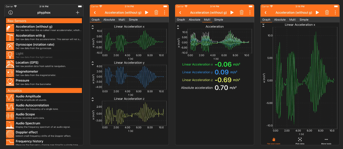
Figure: Phyphox Application Interface (source: AppStore)
One of the newest tools for collecting data for HAR is by using wearable sensors placed on different human body parts. However, it is crucial to attach the device to the suitable locations of the body for wearable sensors because the sensor location on the body has a significant effect on measuring body movements and recognizing activity.
This video shares the technique on how to collect data from wearable sensors. The experiment is presented including an example of the 6 recorded activities (Walking, Walking Upstairs, Walking Downstairs, Sitting, Standing, and Laying down.) with one of the participants. The device is mounted around the waist, which is confirmed by many studies that it can monitor human movements more accurately due to the location of the device being close to the center of the human body.
You can collect the data from the application mentioned above by yourself. After having the data ready, we can now move on to the implementation part.
1.2. Project creation and importing data
Let's create a project first. This tutorial is created as a public use case that will be accessible in read-only mode for all users at that instance. The project will be successfully created when the roles are all set. For more details of projects and roles, see here.
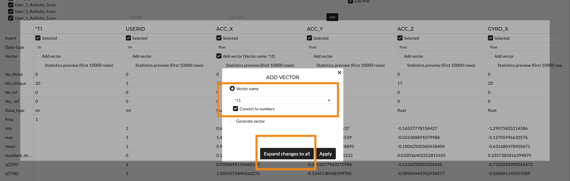
We import our data at the Data Navigation with default configurations. Look at the Import Data description to learn what configurations can be made while importing the data. In our case, we import multiple files with the same structure and content. Additionally, our data is recorded as time-series data with a time column. Precisely, the sampling rate of our dataset is 5hz (or every 0.2 seconds). We can simply apply a time vector while importing by clicking 'expand changes to all' as shown in the below figure.
Optionally, we want to visualize overall activities. We concatenate folders for this purpose in the [crop, concatenate & rearrange the tab in the Data Wrangling section. We choose to concatenate folders methods and save them in the 'concat' folder for later use.

1.3. Exploratory Data Analysis
Let's explore our dataset. We have uploaded the data which in turn yields us 30 different folders with the same data structure.
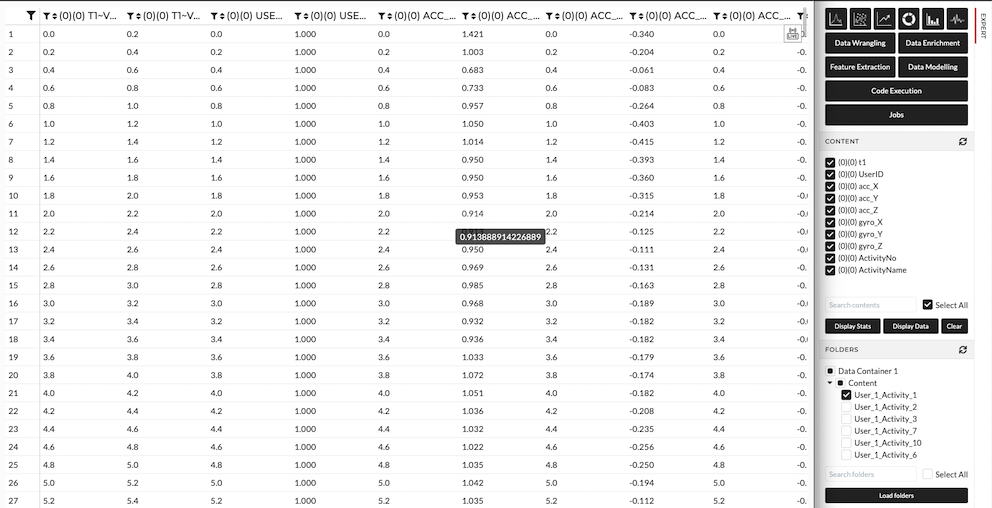
Figure: Display Data
1.3.1. Data Exploration:
Each file contains the following features. Before building any model, understanding the dataset is always a crucial starting point. We will look now at the description of each feature.
| Feature | Description |
|---|---|
| t1 | Time-domain signals were captured at a constant rate of 5 Hz or 0.2-sec duration. |
| UserID | ID numbers of each user. In this case, we have one experiment per participant. There is no need for experiment number ID). |
| acc_XYZ | Accelerometer 3-axial raw signals (acc_Z, acc_Y, and acc_Z). |
| gyro_XYZ | Gyroscope 3-axial raw signals ( gyro_X, gyro_Y, gyro_Z). |
| ActivityNo | Number of activities ranging from 1 to 12. |
| ActivityName | Name of activities including the following activities; walking (1), walking-upstairs (2), walking-downstairs (3), sitting (4), standing (5), lying (6), stand-to-sit (7), sit-to-stand (8), sit-to-lie (9), lie-to-sit (10), stand-to-lie (11), lie-to-stand (12). |
1.3.2. Exploratory Data Analysis (EDA)
Primarily, EDA is the step we perform to gain insight from the data that can tell us beyond the formal modeling. Additionally, we can also avoid the common pitfall such as the law of small numbers or biases that might occur based on our past knowledge. In other words, we might find some relationship between features that might surprise us leading to a more interesting hypothesis formulation later on.
We will start with the general plotting at Transient viewer, which is specially designed for time-series data or line plot visualization. Our data have time vectors which will be shown on the x-axis. We visualize different activities as an example. If we visualize all of the activities the different patterns can be categorized into three groups. 1. Basic activities; walking (1), sitting (4), standing (5), and lying (6). 2. Dynamic activities; walking upstairs (2), walking downstairs (3) 3. All postural transitions activity; stand-to-sit (7), sit-to-stand (8), sit-to-lie (9), lie-to-sit (10), stand-to-lie (11), and lie-to-stand (12).
| Acceleration Signals | Gyroscope Signals | |
|---|---|---|
| Walking |  |
 |
| Walking-upstairs |  |
 |
| Stand-to-sit |  |
 |
| Sit-to-stand |  |
 |
Figure: Transcient View of different activities performed by user 1.
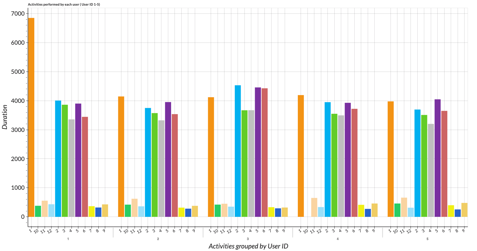
We can visualize overall activities with our descriptive plot at the Descriptive Viewer. We take all users into account. As a result, we can see that the basic and dynamic activities have more records than those of transition activities. With the descriptive viewer, we can analyze and compare all activities performed by each user with a combined bar chart.
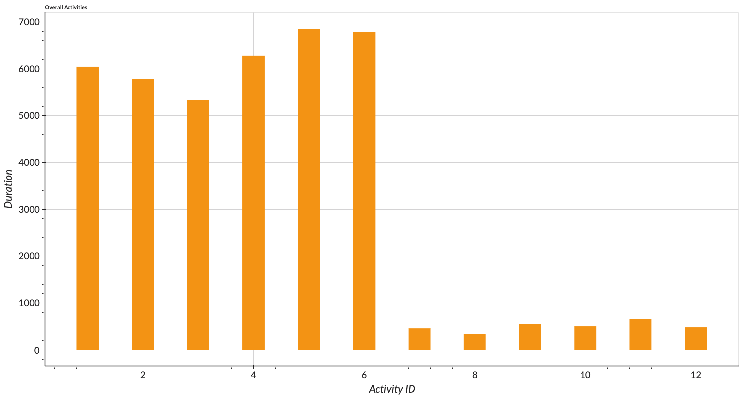
Figure: Descriptive of all activities performed by all users visualized with bar chart.
| User 1 - 5 | User 25 - 30 |
|---|---|
 |
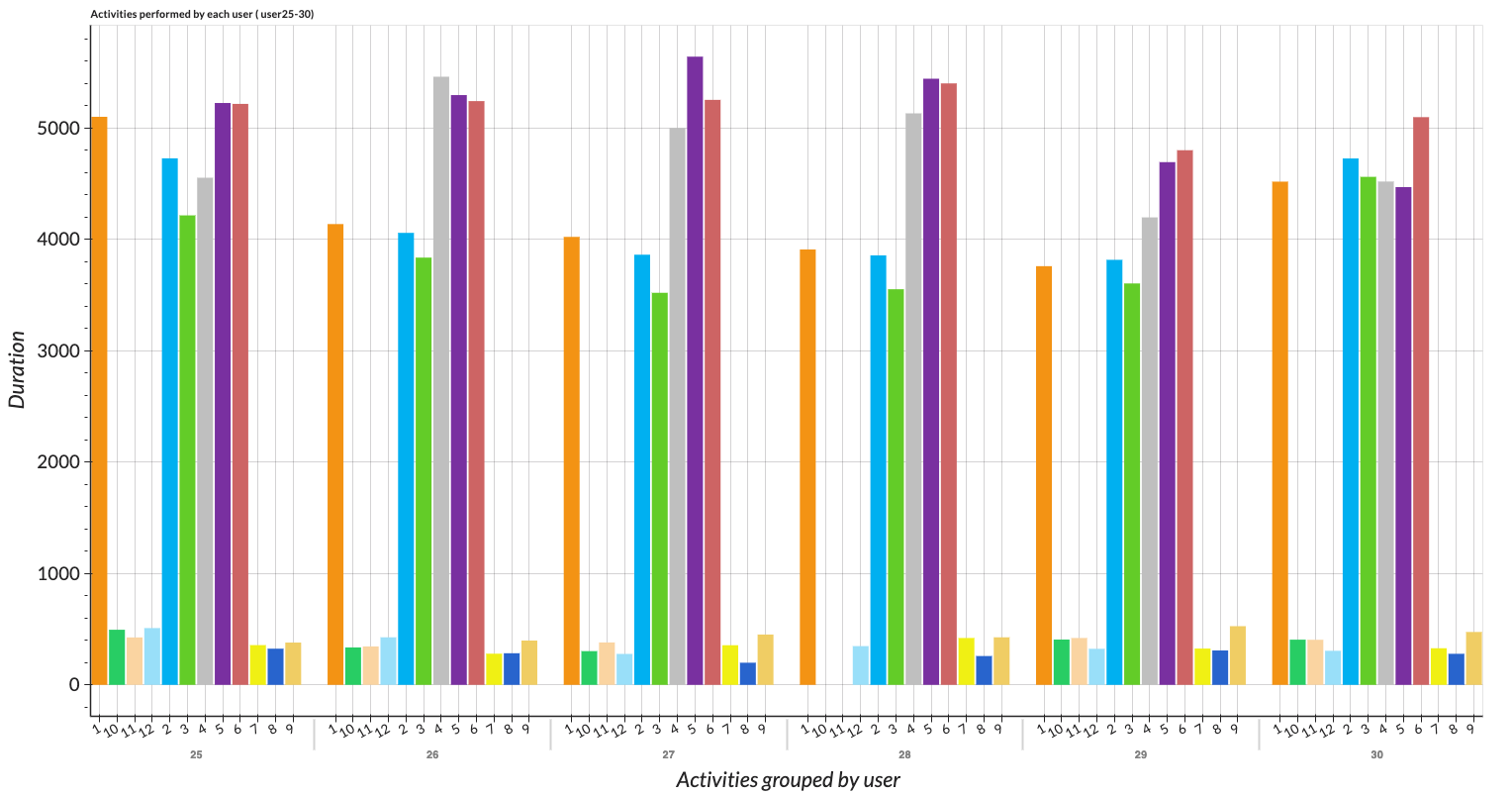 |
Figure: Descriptive of all activities performed by each user visualized with combined bar.
1.4. Splitting Train/Test Data
Besides splitting train and test data for model building, we want to also build the Live App that will process original data into the output with our pipeline module. Therefore, in this tutorial, we would split the data from the beginning before pre-processing our data. For simplicity's sake, we will perform feature extraction and split the data at the same time so we can save time and no additional folders need to be created. We will split train/test data by UserID 1-28 and 29-30 respectively.
1.5. Feature Exngineering
1.5.1. Feature Extraction
Feature extraction can be seen as a data pre-processing step where different kinds of features will be extracted from the raw data. In the first step, the raw data (time series) will be split into short intervals - windows. Let's start extracting the features.
At the 'Feature Extraction' tab, we will set our first setting. Here we will try a wide range of features. First of all, we select all data content on the right of all users we want to include in the training set which is the folders of UserID 1 - 28. For the feature extraction setting, the special thing about this function is we do not have to select every signal from every folder. We can just select from one folder and apply it to other folders all at once. We set chunk width to 15 and set 'Track chunks as feature'. This is considered a 3-second window since our data's sampling rate is 5Hz.

Figure: Example of the chunk width setting.
For the column chunking, let's just extract here all the possible features. We separate the data into two groups which are shown in the below table.
| Group | Sections | Features |
|---|---|---|
| 1 | Signals: | UserID and ActivityNo |
| Signal type: | raw | |
| Intensity: | Min | |
| Transformation type: | None | |
| 2 | Signals: | acc_XYZ, and gyro_XYZ. |
| Signal type: | raw | |
| Intensity: | predefined features as Minimum | |
| Transformation type: | psd, wavelet_cwt, fft, none | |
Next, we set relative, labeling as count by measurement, and expand to all neighboured folders. Here is important if you want to apply what you have chosen to all other folders as we mentioned earlier. After finishing all the settings, we can calculate the resources needed. The dimension on the right-most box will tell us the needed memory for running this job. In our case, it shows the needed memory of 2.01 GB. When we apply this operation, we set the resources to 2 cores and 24000 MB. Kindly follow our video demonstration for this section.

1.5.2. Data Cleaning
We will clean the missing value if there is any in the replace & remove tab in the Data Wrangling. As our data features have increased to more than 4,000 features. These features are extracted as the settings we specified earlier which means that not all features can be extracted the same way. Some features may have NONE values. We must clean the data first before we can process any further steps.
1.5.3. Feature Selection
In this section, we will demonstrate how to perform feature selections, also known as dimension reduction. There are several techniques to select features for building the model. The filtering method, which calculated the score for all features and selects the features with the best scores, is widely used because it can be applied to almost any kind of data and is not complicated to implement. However, in this tutorial, we will introduce the wrapper method, namely principal component analysis (PCA) which is based on projection, these methods can reduce the dimensions of the feature while maintaining the representation of the features.
We perform Principal Component Analysis (PCA) in this step at the Dimension Reduction tab in the Data Enrichment section. We select all signals excluding unique value (USERID) and dependent variable (ActivityNo). 50 components are selected arbitrarily. We will discuss how to select the suitable numbers of components in the extension section. The PCA elements are saved in the newly created 'Train_v1(PCA)' folder. We copy the ACtivityNo signal to this folder.
1.6. Train Models
Let's switch to the Train Model Tab in the Data Modeling section and apply models to our pre-processed training data which is PCA features.
Then, we set "ActivityNo_raw_1s1_min" as our target. The following models will be trained.
- GaussianNB classifier
- Logistic Classifier
- Decision Tree
The model is configured with a 3-fold cross-validation method with the default setting the ratio of train/val/test dataset is 57:28:15 as the default setting. We will ignore the ensemble options for the moment.
After completing all the settings, the window will appear, in which we can confirm the automatic assumption for the problem type (regression or classification) and the evaluation metrics (accuracy in this case).
The result for this classification task will be shown after the job status changes to finished. When we move the cursor on each model, the confusion matrix will appear on the left where you can check the accuracy for each class. On the right will be the overview of the train/test score.
Figure: Confusion Matrix of the prediction of training set.
From the result shown in the figure above, the logistic classifier model gave the best performance among these three and we will use this trained model for our test data. However, the result does not look good at all. We discuss how to improve our model in an extended version below.
1.7. Discuss model performance
We have trained three models including
- GaussianNB classifier
- DecisionTree Classifier
- Logistic Classifier
Both GaussianNB and DecisionTree classifiers gave us scores that are lower than 60%, while the logistic classifier yields around 70% accuracy.
Let's take a look first at the GaussianNB classifier or Gaussian Naive Bayes classifier. It is one of the Naive Bayes classifier families. The algorithm applies Bayes’ theorem with the “naive” assumption of conditional independence between every pair of features and it assumes that the presence of a particular feature in a class is independent of other features. The GaussianNB is an extension of this algorithm referring to the Gaussian or normal distribution of the data. We might notice that if we visualize our data, each class is not distributed normally which could affect our model's performance as we have seen. However, the good thing about this algorithm is that it is faster than other advanced algorithms, especially with large data.
The second model is the Decision Tree classifier whose structure is treelike and comprised of nodes and branches. The decision tree works well on a small dataset. For a large dataset, it requires more settings for the model to perform well enough such as setting maximum tree depth or pruning. Additionally, the algorithm is sensitive to noise and is prone to overfitting. The model did not perform which could be a result of many features fed into the model. As mentioned, the larger the data or the more features we have, the algorithm needs to be set properly.
The last model is Logistic Classifier which is mostly known for binary classification, but the algorithm is also applicable for multiclass as well. This algorithm cannot handle pure categorical data or string format. In this tutorial, we already excluded the string features 'ActivityName' and use only 'ActivityNo'. Therefore, our data works fine with the model. Additionally, the model can handle colinearity or the situation where there is a correlation between features. We are aware that collinearity and multicollinearity are not the same, and the model will not be able to perform well in the latter situation. Additionally, the model is less likely prone to overfitting, especially when we applied already a dimension reduction in the earlier step. More information about the logistic regression classifier for multiclass can be found here and here.
Consequently, the Logistic Classifier yield accuracy of over 70% which we will use to apply for test data. Yet, the performance can still be improved which we will discuss in the later section here.
1.8. Pre-processing Test Data for Live-App Building
We have separately pre-processed the train set, now we apply the same operations for test data. We could have just processed them together at the beginning. However, we would like to apply our operations for test data for our Live App. Therefore, in this section, we will highlight how to pre-process test data for later use in the Live-App building.
We start from feature extraction of users 29 and 30. The process and the setting are the same as what we have done for training data. The difference here is instead of permanently saving the jobs, we will process every operation for test data with the 'preview' option.
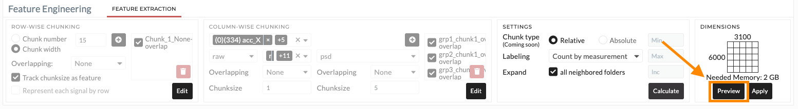
Figure: Preview Option for Results Viewing
This is a crucial step if you want to apply the operations later for the story and live-app building. As shown in the figure below, we only hit the 'preview' button for every operation we perform for test data. Once FE is done, we open the job and click the 'load result' button, so that we can further perform the dimension reduction operation directly on this output.
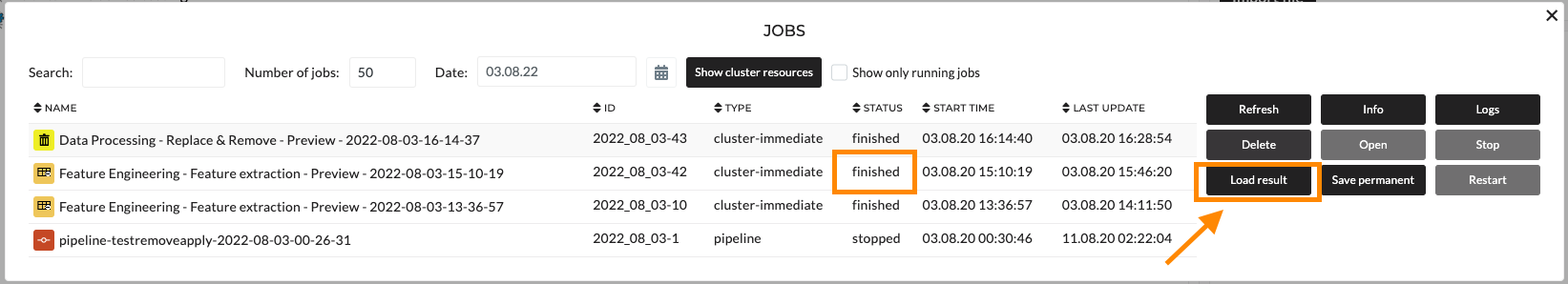
Figure: Loading Result of the Finished Operation
We first go to the job status section and click the load result button. The output of the feature extraction operation will appear in the folder area. We repeat all the steps with the preview option including replace&remove and dimension reduction (PCA).
Interestingly, we can perform dimension reduction by using the saved parameters of PCA performed on train data. Let's load the job of PCA we performed on train data and apply it to our test set. Instead of selecting 'tranform' as previous, select 'retransform' and apply the PCA model. You can see that the setting is set and frozen. We have to match the features, else the platform will not allow you to perform any step further.
1.9. Apply Model to Test Data
To apply the model, let's switch to the Apply Model Tab in the Data Modeling. We can select our final model performed with our train data, and select the result of PCA features that we have just processed. We can now apply the operation and let's discuss the result in the next section.
Additionally, we want to visualize our prediction. We switch to the correlation section and select the first 3 PCA components and color these data points with our prediction. Let's add comments to these operations so we do not forget which operations we would like to add to our story. For instance, right-click on the operation and select the 'add comment' button. On the left side of the screen, you will see the blank space where you can insert comments for each operation.
1.10. Story Creation for Live-App
We create the story in the story section. Once the story is created, we will add the operations to our story. On the right-hand side of the screen, there is a list of the history that we performed for our data. We will select those operations performed in the previous section (for test data). Luckily, we have added comments to those operations so we can find them easily.
The operations will appear on the left side of the window. We can expand our stories for the view of the operations level. To execute our story, we must apply our story first. Here, we can apply it temporarily. After applying the story, we can re-apply again to change the input data if needed. The pop-up window will appear asking if you want to change the data input. Here, you can easily replace the data if you wish to change the data for this story.
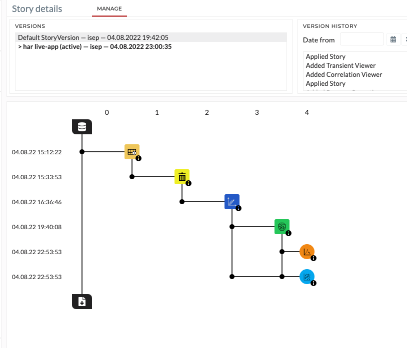
Figure: Story details for test data
1.11. Live App building
In this section, we will demonstrate how to build an App with Apply model Story, including the steps:
- Notification System
- Dashboard
We duplicate the story to avoid editing the original one. With duplicated version, we can edit or customize our story without changing the original version. We keep the operation we need. We add later on the 'math and logical' part for calculating our test score to see our model performance.
Let's start building our application. First, I switched to the App module and created an App called HAR Live-App. We set the title and image, and insert user management for this application as usual. Once we enter the second page, we can still customize our story to match our analytic workflow's purpose. On the same page, we set the notification system. For this tutorial, we set the notification system to notify email whenever activity 4 (sitting) is reported.
On the next page, we build here our dashboard. All the plot elements we have added to our story can be added to the application. Also, we add standard KPI and Gauge elements into it. The preview section will present the interface example of our dashboard. It can be modified simply by pressing Shift+Q key on the keyboard. See here for more details about the App, Dashboard, and notification system.
1.12. Publishing the Live App.
TBD
Reference:
- Feature Analysis to Human Activity Recognition. Available HERE